Andy White Anthropology
  • Home
  • Research Interests
    • Complexity Science
    • Prehistoric Social Networks
    • Eastern Woodlands Prehistory
    • Ancient Giants
  • Blog
  • Work in Progress
    • The Kirk Project >
      • Kirk 3D Models list
      • Kirk 3D Models embedded
      • Kirk 2D images >
        • Indiana
        • Kentucky
        • Michigan
        • Ontario
      • Kirk Project Datasets
    • Computational Modeling >
      • FN3D_V3
    • Radiocarbon Compilation
    • Fake Hercules Swords
    • Wild Carolina >
      • Plants >
        • Mosses
        • Ferns
        • Conifers
        • Flowering Plants >
          • Grasses
          • Trees
          • Other Flowering Plants
      • Animals >
        • Birds
        • Mammals
        • Crustaceans
        • Insects
        • Arachnids
        • Millipedes and Centipedes
        • Reptiles and Amphibians
      • Fungi
  • Annotated Publications
    • Journal Articles
    • Technical Reports
    • Doctoral Dissertation
  • Bibliography
  • Data

An Update on the Kirk Project

3/6/2017

5 Comments

 
Without thinking about it too hard, it seems like a disproportionate amount of my work on the early hunting-gathering societies of the Eastern Woodlands has been done in the company of sick children. Today's update on the Kirk Project comes to you from a crowded chair, with my typing arms constrained by the presence of a 3-year-old in pajamas watching Fireman Sam. For the full effect, play this in the background while you read this post.

I have four updates, one of which includes an apology.

Picture
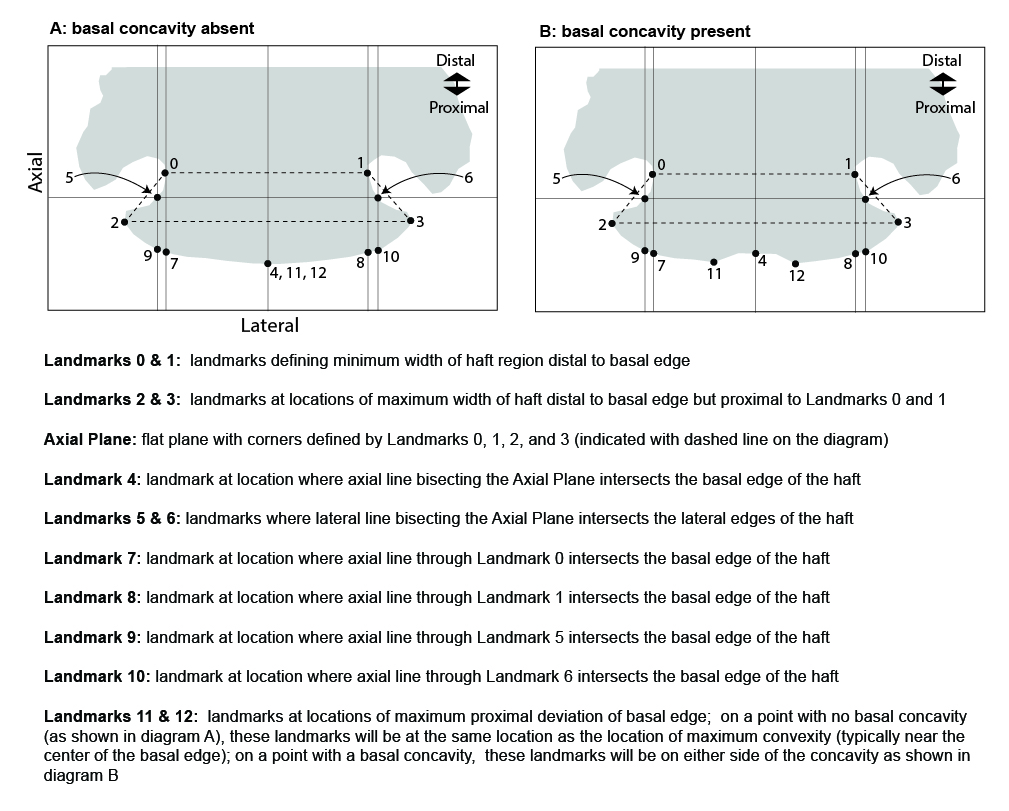
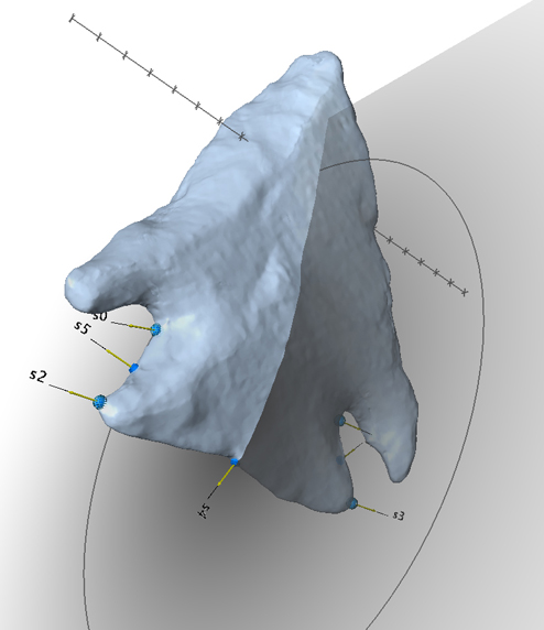
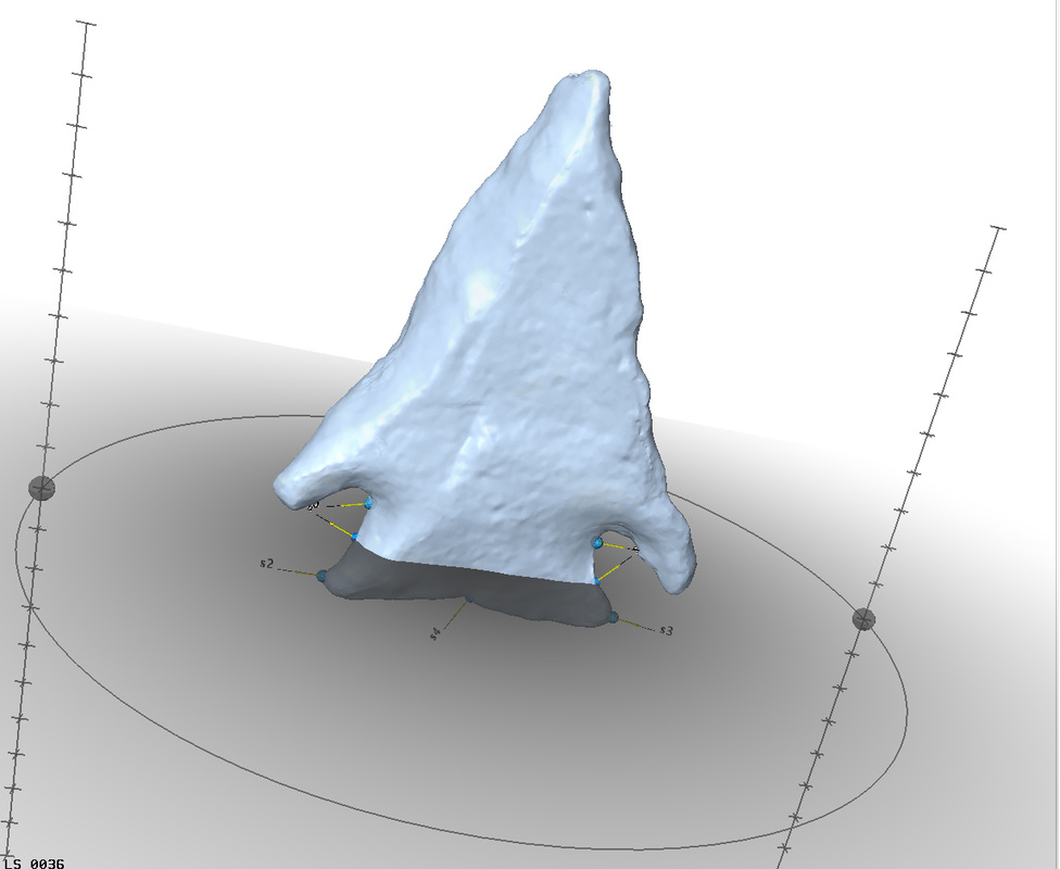
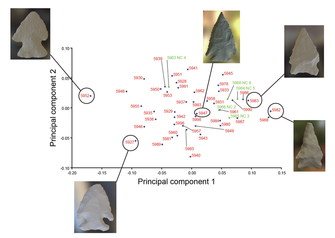
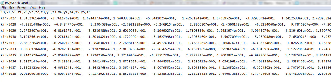
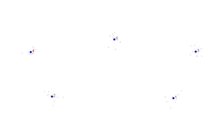
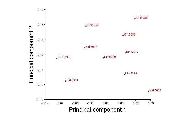
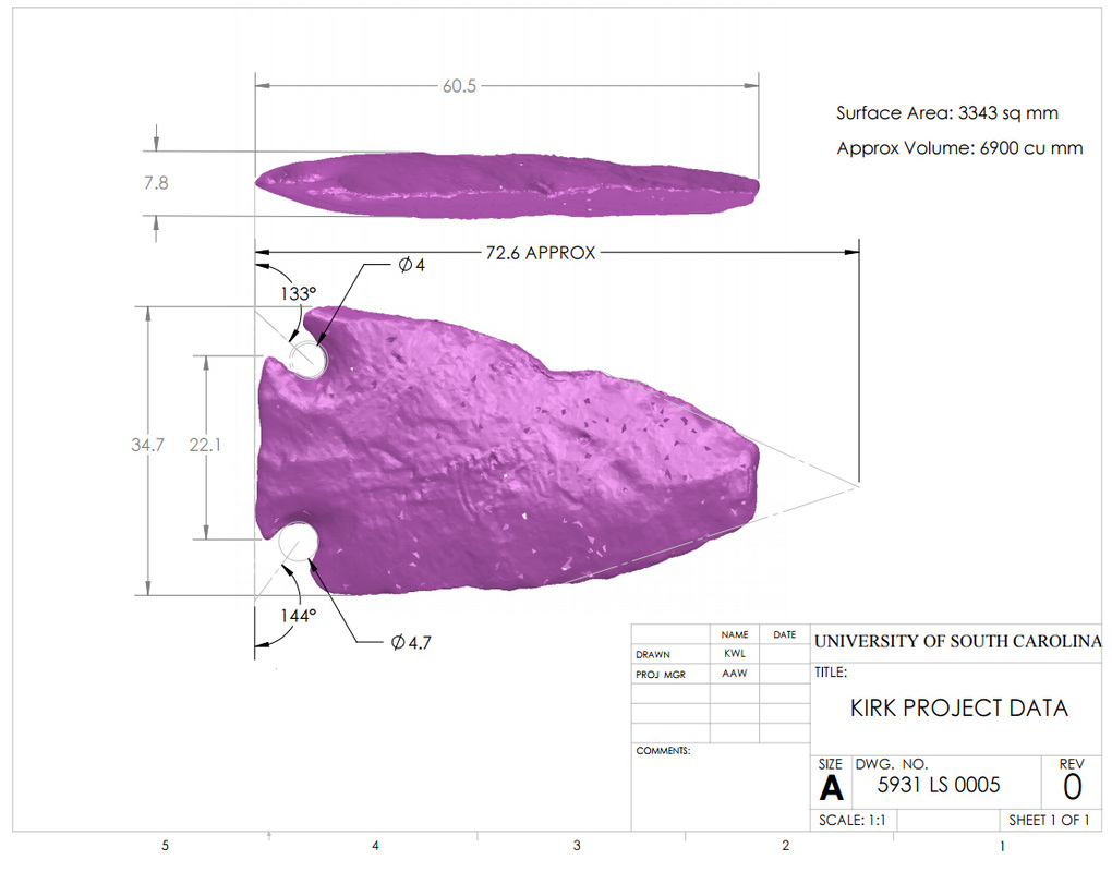
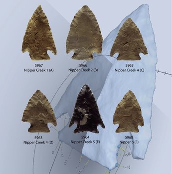
South Carolina Antiquities Paper

The first salvo of analysis related to the Kirk Project comes in the form of a paper in South Carolina Antiquities titled "A Preliminary Analysis of Haft Variability in South Carolina Kirk Points." The paper uses morphometric data from 46 Kirk points, considering shape variability in the haft regions and asking which dimensions of that variability are most likely to be linked to change through time. The majority of the points are from the Larry Strong collection (from Allendale County, South Carolina), a surface assemblage that was presumably created over a long span time of time. I compare variability in the Larry Strong points to variability in points from the Nipper Creek cache (Richland County, South Carolina), which was presumably created over a very short period of time. You can find a link to the paper on my Annotated Journal Articles page. Eventually I'll add files with the data I used in the analysis.

Picture
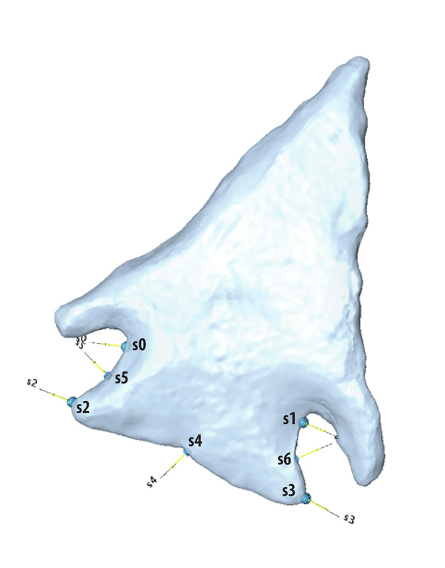
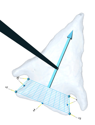
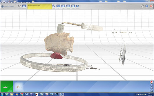
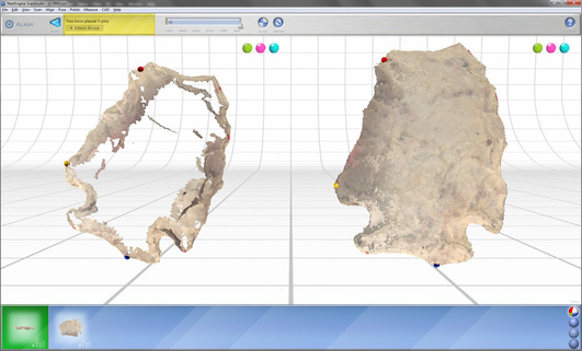
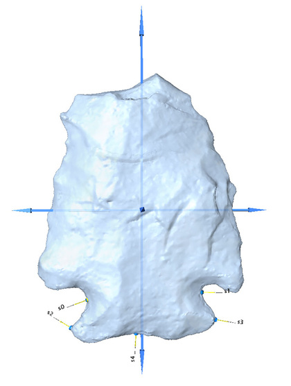
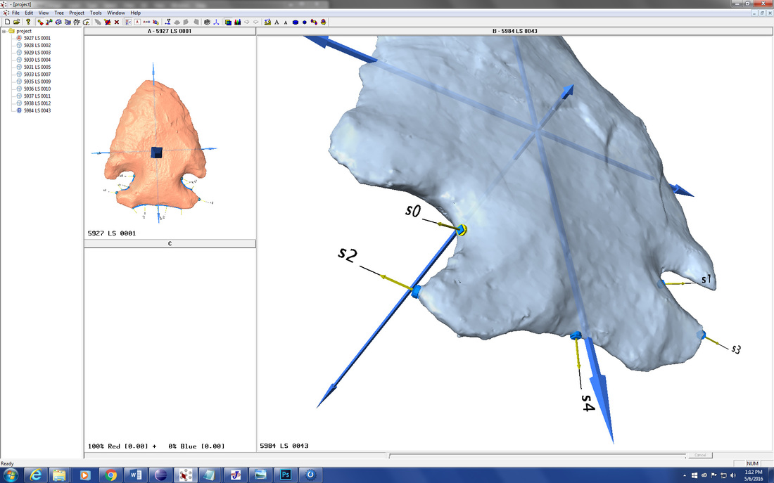
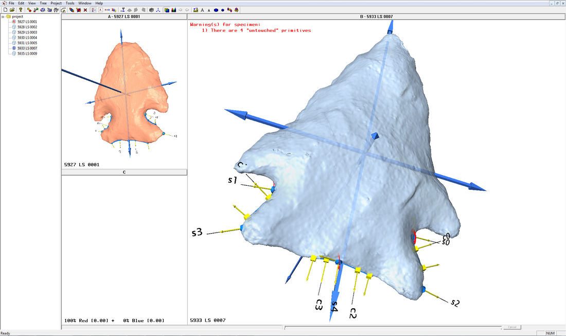
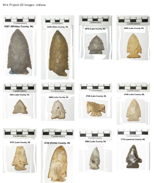
Morphometric Analysis on Two Tracks

Although based ultimately on 3D models, the analysis in the South Carolina Antiquities paper was done in 2D. I will continue working with the 3D models I'm producing, finding ways to capitalize on the richness of those data. At the same time, however, I plan to pursue a large scale 2D analysis that will allow me to make use of the large amount of data that I collected for my dissertation.  I've begun organizing and posting the "rough" scaled images of Kirk points from my Midcontinental data set by state here. It will take me a while to get all those photos in order, as there are over 600.

Once the images are assembled, I will be able to extract and analyze comparable 2D shape data from all the Kirk points in my dataset. At that point, we can finally start addressing questions about patterns of Kirk variability across large expanses of space. With a system in place, it will be much easier to feed new points from other regions into the analysis. That brings me to my next update . . .

Picture
Apologies for My Sluggishness, Alabama . . . and Tennessee . . . and Georgia . . .

As I wrote several weeks ago, a mention of the Kirk Project in the newsletter of the Alabama Archaeological Society spurred several people to contact me about their collections. I have continued to get emails, but I haven't yet started assembling them in an attempt to take advantage of the offers for help and information. Starting to get back to people is next on my "to do" list today. I truly appreciate the communication, and I apologize for not responding to everyone in a more timely manner. The  "zero inbox" grail has always eluded me. It's a personal failing.

Picture
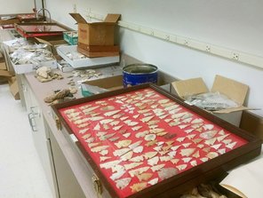
Processing a Large Collection from Aiken County, South Carolina

Over the holiday break, SCIAA received a large, donated artifact collection from Aiken County, South Carolina. Processing the entire collection (which has taken over much of my lab) is a long term proposition. One of our highest priorities is inventorying and labeling the Paleoindian and Early Archaic materials so that we (by "we" I mean primarily Al Goodyear, Joe Wilkinson, and myself) can include them in analyses. Look for those materials to be incorporated into the Kirk Project in the future.


5 Comments

In Press: "A Preliminary Analysis of Haft Variability in South Carolina Kirk Points"

11/28/2016

0 Comments

 
The gears of science almost always turn more slowly then I would like. It was about a year ago that I first hatched the idea of the Kirk Project, and I've just now submitted my first formal publication related to describing and understanding variability in Kirk points from the Southeast.  The paper, titled "A Preliminary Analysis of Haft Variability in South Carolina Kirk Points," will be published in the next issue of South Carolina Antiquities.

The paper considers haft variation in a sample (n = 46 total) of Kirk points from the Larry Strong Collection (n = 41, Allendale County, South Carolina) and the Nipper Creek cache (n = 5, Richland County, South Carolina). The Larry Strong portion of the sample is a large "long time” assemblage that contains Kirk points from the full range of time those points were produced in the region. The Nipper Creek cache, in contrast, is a “short time” assemblage that was produced during a small window of time.  Comparison of these assemblages can be used to explore which aspects of haft morphology may be carrying useful stylistic information that is sensitive to change through time and, potentially, patterned in ways that can eventually tell us something meaningful about Kirk societies. This table summarizes the sample and provides links to the downloadable 3D models that I used (I also posted the table on my Data page). 

My analysis focuses on various aspects of shape as characterized by a series of landmarks placed on 3D models. Although 3D models are the starting point, I purposefully performed the preliminary analysis in the paper in only two dimensions (i.e., utilizing just the shape of the outline of the haft region and getting rid of data related to thickness).
Picture
The main take-away point from the paper is that shape variation in the lateral haft margins appears to be a better candidate for capturing stylistic change through time (and potentially also stylistic variability across space) than the the morphology of the basal edge and the overall length:width proportions of the haft. The "short time" Nipper Creek assemblage is more consistent in the degree of haft flare and shape of the lateral/basal junction than the "long time" Larry Strong assemblage, which is what one would expect if design of the lateral haft margins was strongly influenced by some kind of cultural-bound choice (i.e, if lateral haft morphology is essentially isochrestic). This is a potentially important observation, as basal edge shape and treatment are often thought to be good attributes upon which to base “type” distinctions that are presumed to have temporal significance. While basal edge morphology appears to account for the greatest amount of variability overall in the shape analysis, it may not be strongly linked to style within the Kirk Corner Notched cluster (and may, in fact, be linked to function through haft repair and maintenance). It will be important to sort this out going forward to avoid inclusion of non-stylistic variability in a stylistic analysis.

I'll let you know when the paper is available. In the meantime, I'll be working on expanding the analysis in several different directions. I'm hoping that making my primary data sources (i.e., the 3D models) available as freely downloadable files will encourage others to do the same. We're really not doing ourselves any favors by not taking better advantage of the data-sharing potential offered by the digital age.

Funds to support inventorying and analysis of the Larry Strong Collection were provided by the Archaeological Research Trust.
0 Comments

Some Very Preliminary Kirk Morphometric Data

10/4/2016

14 Comments

 
I've spent some time over the last few days generating some basic morphometric data from the 3D models of Kirk points that I've processed so far (n = about 50) . I'd like to have about double that for a formal analysis to publish, but I also would like to discuss some preliminary results as part of my presentation at the SEAC (Southeastern Archaeological Conference) meeting that's coming up in a few weeks. So you go to war with the Kirk assemblage you've got, not the Kirk assemblage you want.

Before I talk about the data, I'd like to congratulate myself on having the forethought to take a day last spring to write down the workflow right after I got it figured out. There were a few details that I neglected to mention in that blog post, but overall it was a huge time saver. Figuring out the steps was enough of a pain-in-the-ass the first time. Let us never do it again.​

Picture
I defined seven landmarks on each point (s0 through s6).

​To define these landmarks consistently, I first oriented the point to minimize the horizontal distance between s0 and s1. Generally, that resulted in s0 and s1 falling on roughly the same plane. I then defined s2 and s3 to mark the maximum deviation of the lateral haft edges proximal to maximum constriction of the haft (marked by s0 and s1).  

Picture
I used s0, s1, s2, and s3 to define the axial plane (in the "View" pulldown menu). This superimposes an asymmetrical grid on the point and defines a set of three planes: axial, coronal, and sagittal (named following conventions for anatomy, which is what this software was designed for). 

Picture
I turned on the sagittal plane to locate landmark s4. The sagittal plane splits the axial plane down the middle. Landmark s4 is defined as the location where the sagittal plane intersects with the basal edge of the point when the sagittal plane bisects the axial plane. If the point is symmetrical, s4 will fall in the center of the basal edge.

Note: the sagittal plane is movable. When you initially turn it "on," it's automatically centered in reference to the axial plane. If it gets moved you can recenter it simply by turning it off and then on again.

Picture
Finally, I turned on the coronal plane to locate landmarks s5 and s6. Landmarks s5 and s6 are defined as the locations were the coronal plane intersects the lateral edges of the haft when the coronal plane bisects the axial plane.

For each point, you have to tell the software how the landmarks correspond to those on the "atlas" model. The simplest thing to do is to always place the landmarks in the same order. You still have to manually define the correspondence between each model and the atlas ("View Correspondences" in the "View" menu).

I followed the same steps I described in the previous post to export and edit the data so that I could import it into MorphoJ. I used MorphoJ to perform a principal components analysis (PCA), the purpose of which is take all the variability in the 3D data and boil it down to its most important components. PCA lets you flatten the variability in a dataset into scores that you can plot in two dimensions.

Here are the basic results of the PCA performed on the points currently in the sample:
Picture
I haven't spent any significant time digging into the data yet, but my initial reaction is that the first principal component may well be measuring variability related to time. If you look at the examples of points that fall at the far left end of the plot, they look very Taylor- or Thebes-like, with relatively long hafts, deep notches, and small/shallow basal concavities/indentations separating broad convex basal edge segments. The points at the far right of the plot, conversely, have relatively short hafts, shallow notches, and broad basal concavities. If you squint a little, maybe, you can see how that end of the Kirk spectrum is trending toward a bifurcate/lobed haft morphology. In the center of the plot are points like 5947, which I think we can agree is a "modal" Kirk Corner Notched.

With the exception of the Nipper Creek cache points (shown in green), all the points in the sample are from Allendale County, South Carolina, and are made from Allendale chert. This all but eliminates the possibility that the variability is due to space or raw material.

My next step is to explore the possible "time" component of the PCA by gathering some data from the point forms that bracket Kirk: Taylor (on the earlier side) and lobed/bifurcate points (on the later side). If I'm correct that the first principal component shown above is telling us something about time, the Taylor points should plot to the left and the bifurcate/lobed points should plot to the right.  It's notable that four of the five points from the Nipper Creek cache plot close together. Those points were almost certainly produced during a short period of time (but so was 5963 NC 4, so . . . something to think about).
14 Comments

Kirk Project: Workflow from Point to 3D Morphometric Data

5/6/2016

2 Comments

 
I've spent most of today and yesterday trying to find a workflow path that gets me from the collection of 3D data (which I've been doing for months now) to a set of numbers that I can do meaningful analysis on.  This has involved, mostly, a lot of trial and error with various software programs. I think I've finally found a series of reasonable steps that will let me go from the 3D models to characterizations of shape data that I can examine visually and statistically.

This is post is mostly a way to document these steps for my own benefit, so that I can refer back to them in a week or a month when I've forgotten what I just figured out. This may not be the final procedure that I end up using for a large scale analysis. I'm putting this out there in public in case anyone finds it useful. Or in case I get hit by a bus and someone else needs to carry on with this important work.
Acquiring 3D Data
PictureScan in progress.
I'm using a NextEngine Desktop 3D scanner (UltraHD, Model 2020i). I'm scanning each point in two orientations: (A) one that exposes all the edges and (B) one that exposes the faces. Before scanning, I use a red pen (supplied with the scanner) to place a series of small dots along the edges of the point. These dots are used to align scan sets A and B into a single model (three points are required for alignment), so they should be placed in locations likely to show up in both scans.

I'm using the autodrive (rather than the multidrive) to rotate the points as they are scanned. I use part of an eraser to elevate the point off of the platform, and the padded to gripper to hold it firmly in place without damaging it.

For each scan set, I've got the scanner set to rotate the point through 10 divisions at the middle HD setting (67k points/square inch).  This may be overkill, but it's been working so far and I've been producing models far faster than I've been processing them (I've scanned about 90 points but have only processed the models for about 40). I scan with texture capture on, because I need to be able to see the red dots to do the alignment.

Processing 3D Data
PictureExample of raw scan data.
I keep copies of the raw (unprocessed) scan data in an archive folder. At the settings I'm using, the raw data for a set of scans from a single point occupies about 300-450 MB. I copy the files for each point and put them in a "processing folder."

​Processing is done in the ScanStudio software that came with scanner. The first thing I do is trim away the non-point things that were captured in the scan. This is a simple operation: you just select what you don't want and delete it. Because I'm scanning in two different orientations, it doesn't matter if a small bit of the actual point gets deleted where it's touching the eraser and gripper - data for those areas will be contained in the other set of scans.

PictureAlignment in process.
After the two sets of scans are trimmed, I align A and B. This is done by determining which of my red dots I can most reliably locate on both scan sets and marking them with color-coded pins. Again, this is a fairly simple process. I've found that some care in this step can significantly reduce the amount of time you have spend cleaning up the model later. 

After at least three pins are placed (I'm not sure that placing more than three actually leads to better results), you hit the "align" button and see what you get. I find it helpful to switch the display mode to "solid" at this point (removing the photo-like surface texture) because it is much easier to see how the two scan sets actually lined up. If the alignment is bad, you can tell. Sometimes an alignment issue can be mitigated by just going back and re-setting the pins and doing the alignment again. Other times it is apparent that the best solution is to go back to square one and re-generate the raw scan data (i.e., put the thing on the scanner and start over).

PictureFused model.
Assuming the alignment is okay, I fuse the two scan sets together with the "fuse" command. This is a one-button operation.  This is another one button operation. I'm using these fuse settings:
  • Volume Merge,
  • Resolution Ratio 0.5 
  • "Create Watertight Model" unchecked
  • "Include Textures" checked
  • Texture Blending 5 pixels
Fusing scan sets A and B produces a new mesh, conveniently labeled "C." If I'm satisfied with the way C looks, I go ahead and delete A and B at this point.

The fused model requires some clean up. There are often small bits "floating" around the edges and at locations on the surface were data from A and B overlapped. These can be removed using the trim tool. The cleaner the model, the less time this will take, obviously. I really feel like the scanner has good days and bad days: sometimes it seems like the scans are really messy no matter what you do, and sometimes things just work out easily. Regardless, I'm not sweating pixel-level details on these models because it won't affect the kind of morphometric analysis I'm planning on doing. I just need the models to be fairly good approximations of the actual point.

After cleaning up the fused model, I run the "remesh" operation (resolution ratio = 0.9) to fill the holes and even things out a bit. Sometimes this reveals a few more defects that can be addressed through limited trimming. In that case, I'll run the "fill holes" operation ("smooth" and "smooth boundaries" checked) afterward to fill any remaining holes in the mesh.

The file I'm working with to produce these images is about 23 MB at this point. I use the "simplify" tool (set at 0.0050") to reduce the file size to about 5 MB. Then I create a .STL file for exporting the model to Sketchfab and a .PLY file to use for analysis in Landmark.  Here is the model on Sketchfab:

Kirk 5984 by aawhite on Sketchfab

Deriving 3D Landmark Coordinates
This is the part of the equation I just figured out the other day. I discovered the Landmark software package (available here) that allows you position sets of landmarks on the surfaces of 3D models. The software was designed with three-dimensional, irregular biological structures (such as bones) in mind, but will work great for projectile points as well. It is mainly a software to acquire, rather than analyze, coordinate data (at least in my plan). 

Even though the manual says the software will work with .STL files, it didn't seem to want to do it for me. So I converted a batch of 10 Kirk models into .PLY files so I could import them into Landmark and work my way through the process of generating data. I added the model I just created above to the batch to illustrate the steps in this software.
Picture
For a trial run, I defined five replicable landmarks that can be placed in the haft region when the point is orientated with the tip pointing up: the points of greatest constriction (s0 and s1), the points of greatest width below the notches (s2 and s3), and the point of greatest divergence from horizontal along the basal edge (s5). The labels are automatically applied to the points as you place them.

As in other software like this, you place the landmarks in the same order each time because the end result is to going to be a file of numbers with XYZ coordinates corresponding to the locations of those landmarks on each of the objects in your assemblage. The next software that reads that file is going to assume that the coordinates are all in the same order, so they better be or you'll get nonsense back. Landmark helps with this by making the process of applying consistent sets of landmarks to different objects semi-automated.

Here is a close up showing the landmarks placed on the surface of the model. You can use your mouse to drag them around and get them exactly where you want them:


Picture
After I placed the five landmarks on a group of ten Kirk point models, I exported the coordinates of the landmarks by highlighting all the models (listed in the pane on the left) and using the "export" function (in the Project menu). I had to play around with several different options to get a file that would eventually work in the analysis software I found (see below). Supposedly I should be able to export files in a format that can be read directly by MorphoJ, but I couldn't get it to work. I had to export the data in the .DTA format and then just edit the text file myself to a format that MorphoJ could read. The .DTA format has the advantage of being a single file with all the coordinates clearly organized, so editing it was no big deal.

Analysis of 3D Coordinate Data 

Once you have 3D coordinate data, what do you do with them? I was surprised to find that my most beloved data analysis package, JMP, doesn't seem to be able to hand 3D coordinate data. Some of software that can do tricks with 3D data, like EVAN, costs money (which I'd like to avoid spending on a product that I'm not sure is actually going to do what I want it to do).  I downloaded various free software packages and played around with several of them. The one I finally got work is called MorphoJ (available here).

The first trick is getting the 3D coordinate data exported from Landmark to be read properly in MorphoJ. As I said above, this wasn't as easy as advertised (here's the relevant section of the MorphoJ manual). Eventually I gave up on the "easy" route and just edited the data from Landmark into a standard comma-delimited text file using Notepad. For future reference, the input data file should look like this:
Picture
The first line gives MorphoJ the column labels. Each line after that contains data for a single Kirk point: the label of the point, the XYZ coordinates of the first landmark, the XYZ coordinates of the second landmark, etc. Don't put commas at the end of lines, don't put in any tabs, etc.

After you create the data file, you import it into MorphoJ using File-->Create New Project. In the dialog that comes up, click "3 dimensions," select "text" as file type, and then navigate to the text file with the coordinate data. If there are no problems with the import it will tell you so. 

Once the data are in there, they'll show up on the Project Tree. Select the data set, go to the Preliminaries menu, and choose "New Procrustes Fit." This performs a Procrustes analysis that rotates, translates, and scales the objects in space to minimize their differences:
Picture
The graphic above shows the results of the Procrustes analysis, with the numbered points representing the centroids and clouds of smaller points around them representing the spread of actual data values. Notice that the points are flipped vertically and horizontally from the way I showed them in the images above, and also that s0 is now "1," s1 is now "2," etc. The results can be viewed along three different axes.

The Procrustes data can be used to do a Principal Components Analysis, which reduces the three axes down to two.  Here is what that looks like:
Picture
Now we're getting somewhere!  The last hurdle will be to figure out if/how I can export the raw principal component data so I can analyze it in another software package.

Working my way through these steps was a "proof of concept" exercise that I needed to do before scaling the analysis up to the full sample. I've been down a lot of dead ends with software.  I'm hoping this is the combination that gets me to a full-scale analysis. The five landmarks I used for the test run really don't take advantage of the 3D model data that I have, so I'll need to start thinking in three dimensions rather than two. And I still don't know how to make use of the data from curves. Once I get those things sorted out, it will be really interesting to see how variation patterns out with a much larger sample (I'm aiming for 100) from a single county and a single raw material. Based on what I've seen as I've been creating the 3D models, I will be surprised if some component of temporal variation is not detectable.  

And then, of course, I'll need to do about 10,000 more of these to see what's going on in the rest of the country.
2 Comments

My Thursday: Radiocarbon and Kirk

5/5/2016

8 Comments

 
I submitted the final grades for my class yesterday, so barring some kind of last minute disaster, my first academic year at South Carolina is done. I'm spending the last part of the week working on the radiocarbon compilation (which I'll need for my paper at SEAC in the fall), moving forward with analysis for a couple of publications I'm working on, and prepping to go in the field and then give a talk next week. My blog has been getting a lot of traffic related to the posts I wrote about the ethnographic megalithic societies of India and Indonesia last year (most of them should come up if you search on "megaliths").  I wish I had time to look at that stuff again right now, but I don't.

I wanted to post this histogram showing the distribution of the ~9,100 dates (intercepts) currently in the radiocarbon compilation (here's the map of the dates I made yesterday). There's a pretty clear trend of an increasing number of dates through time.  Part of that, I think, almost certainly reflects the emphasis that archaeology in the Eastern Woodlands places on the Woodland and Late Prehistoric/Mississippian societies that largely post-date 2000 RCYBP (and the fact that those societies tend to produce large sites with lots of datable deposits). But I think the chart below, as unrefined as it is, is probably also telling us something very basic about demographic change.  There's an inflection point in the number of dates toward the end of the Middle Archaic period (about 5500 RCYBP) that corresponds in time to when we see (generally) more intensively occupied sites, indicators of decreasing mobility, and increasing use of plants that are later domesticates. Yes, I'm saying intensification.
Picture
Distribution of the RCYBP intercepts of 9,129 radiocarbon dates from the Eastern Woodlands.
I think I've found a path forward that will let me extract morphometric data from the 3D models of Kirk points that I've been producing (I've got 41 models uploaded to Sketchfab so far, with a goal of 100 from Allendale County, South Carolina, to serve as the basis for a paper). I found a software package called Landmark (available here for free) that was developed at UC Davis for use with biological materials (i.e., irregularly shaped things).  It allows you to load in a 3D model, place markers and curves on the surface, and export the coordinates of the points for analysis.  I've spent the day learning how to use the software, and have generated a small data set of five points and four curves from ten of my Kirk point models.  The next step is to figure out how to go from the XYZ coordinates that the software exports into something that I can meaningfully analyze.  I don't think that the data analysis package I use (JMP) will do things like Procrustes analysis and, honestly, I've never attempted to analyze a 3D dataset and will need to do some reading to figure out how to start.  If any of my bioanthropology friends have done this sort of thing with morphometric data from skeletal remains and have some advice, I'm listening. Please do not tell me to learn how to use R.
Picture
Screenshot of a couple of Kirk models in Landmark. The software lets you define a set of landmarks on one item and then semi-automatically transfer them to another. Then you can export the XYZ coordinates that describe the locations of the points and, somehow, can be used to describe the shapes of curves that are defined.
8 Comments

One Procedure for Generating Linear Measurements from 3D Models

4/6/2016

1 Comment

 
Things are busy as usual around here, so I don't have time to write much myself today. I wanted to make available to you, however, a nice document produced by Ken Lentz.  Lentz took it upon himself to explore how to go from the 3D models that I'm producing for the Kirk Project to a set of linear measurements. As I wrote recently, getting those linear measurements is something I'm going to need to start doing again in short order. I used a freeware landmark-based program (tpsDIG, which I see is still available here) to derive linear measurements from images for my disseration. The program worked fine, but it was a bit labor intensive and I'm hoping to find an alternate path to getting the same measurements that takes advantage of the fact that I've got a detailed, scaled 3D model sitting right there in front of me. 

Lentz succeeded in getting linear measurements (including angles, which I would really like to be able to measure) from a CAD program, but he had to go through a lot of time-consuming steps to do it.  I'm grateful for his efforts, as I have had zero time myself to seriously explore the issues involved in going from 3D back to 2D. Thanks, Ken, for all your work on this (and taking the time to explain what you did).
Picture
1 Comment

A Test 3D Model of a Kirk Corner Notched Point

2/8/2016

6 Comments

 
Okay . . . I'm making some headway. Some of my 3D model creation issues are beginning to yield to good old-fashioned trial-and-error, and I've uploaded a test model to Sketchfab.  The original is a Kirk Point from Allendale County, South Carolina.  I didn't do full color capture on it, but I'll try one of those next.  Take a look at the model and see what you think.

Kirk 5947 (Allendale SC) by aawhite on Sketchfab

6 Comments

    All views expressed in my blog posts are my own. The views of those that comment are their own. That's how it works.

    I reserve the right to take down comments that I deem to be defamatory or harassing. 

    Andy White

    Follow me on Twitter: @Andrew_A_White

    Email me: andy.white.zpm@gmail.com

    Enter your email address:

    Delivered by FeedBurner


    Picture

    Sick of the woo?  Want to help keep honest and open dialogue about pseudo-archaeology on the internet? Please consider contributing to Woo War Two.
    Picture

    Follow updates on posts related to giants on the Modern Mythology of Giants page on Facebook.

    Archives

    January 2023
    January 2022
    November 2021
    September 2021
    August 2021
    March 2021
    June 2020
    April 2020
    March 2020
    January 2020
    December 2019
    November 2019
    October 2019
    September 2019
    May 2019
    April 2019
    January 2019
    December 2018
    November 2018
    October 2018
    September 2018
    August 2018
    July 2018
    June 2018
    May 2018
    April 2018
    March 2018
    February 2018
    January 2018
    December 2017
    November 2017
    October 2017
    September 2017
    August 2017
    July 2017
    June 2017
    May 2017
    April 2017
    March 2017
    February 2017
    January 2017
    December 2016
    November 2016
    October 2016
    September 2016
    August 2016
    July 2016
    June 2016
    May 2016
    April 2016
    March 2016
    February 2016
    January 2016
    December 2015
    November 2015
    October 2015
    September 2015
    August 2015
    July 2015
    June 2015
    May 2015
    April 2015
    March 2015
    February 2015
    January 2015
    December 2014
    November 2014
    September 2014
    August 2014
    June 2014
    May 2014
    April 2014
    March 2014

    Categories

    All
    3D Models
    AAA
    Adena
    Afrocentrism
    Agent Based Modeling
    Agent-based Modeling
    Aircraft
    Alabama
    Aliens
    Ancient Artifact Preservation Society
    Androgynous Fish Gods
    ANTH 227
    ANTH 291
    ANTH 322
    Anthropology History
    Anunnaki
    Appalachia
    Archaeology
    Ardipithecus
    Art
    Atlantis
    Australia
    Australopithecines
    Aviation History
    Bigfoot
    Birds
    Boas
    Book Of Mormon
    Broad River Archaeological Field School
    Bronze Age
    Caribou
    Carolina Bays
    Ceramics
    China
    Clovis
    Complexity
    Copper Culture
    Cotton Mather
    COVID-19
    Creationism
    Croatia
    Crow
    Demography
    Denisovans
    Diffusionism
    DINAA
    Dinosaurs
    Dirt Dance Floor
    Double Rows Of Teeth
    Dragonflies
    Early Archaic
    Early Woodland
    Earthworks
    Eastern Woodlands
    Eastern Woodlands Household Archaeology Data Project
    Education
    Egypt
    Europe
    Evolution
    Ewhadp
    Fake Hercules Swords
    Fetal Head Molding
    Field School
    Film
    Florida
    Forbidden Archaeology
    Forbidden History
    Four Field Anthropology
    Four-field Anthropology
    France
    Genetics
    Genus Homo
    Geology
    Geometry
    Geophysics
    Georgia
    Giants
    Giants Of Olden Times
    Gigantism
    Gigantopithecus
    Graham Hancock
    Grand Valley State
    Great Lakes
    Hollow Earth
    Homo Erectus
    Hunter Gatherers
    Hunter-gatherers
    Illinois
    India
    Indiana
    Indonesia
    Iowa
    Iraq
    Israel
    Jim Vieira
    Jobs
    Kensington Rune Stone
    Kentucky
    Kirk Project
    Late Archaic
    Lemuria
    Lithic Raw Materials
    Lithics
    Lizard Man
    Lomekwi
    Lost Continents
    Mack
    Mammoths
    Mastodons
    Maya
    Megafauna
    Megaliths
    Mesolithic
    Michigan
    Middle Archaic
    Middle Pleistocene
    Middle Woodland
    Midwest
    Minnesota
    Mississippi
    Mississippian
    Missouri
    Modeling
    Morphometric
    Mound Builder Myth
    Mu
    Music
    Nazis
    Neandertals
    Near East
    Nephilim
    Nevada
    New Mexico
    Newspapers
    New York
    North Carolina
    Oahspe
    Oak Island
    Obstetrics
    Ohio
    Ohio Valley
    Oldowan
    Olmec
    Open Data
    Paleoindian
    Paleolithic
    Pilumgate
    Pleistocene
    Pliocene
    Pre Clovis
    Pre-Clovis
    Prehistoric Families
    Pseudo Science
    Pseudo-science
    Radiocarbon
    Reality Check
    Rome
    Russia
    SAA
    Sardinia
    SCIAA
    Science
    Scientific Racism
    Sculpture
    SEAC
    Search For The Lost Giants
    Sexual Dimorphism
    Sitchin
    Social Complexity
    Social Networks
    Solutrean Hypothesis
    South Africa
    South America
    South Carolina
    Southeast
    Stone Holes
    Subsistence
    Swordgate
    Teaching
    Technology
    Teeth
    Television
    Tennessee
    Texas
    Topper
    Travel
    Travel Diaries
    Vaccines
    Washington
    Whatzit
    White Supremacists
    Wisconsin
    Woo War Two
    World War I
    World War II
    Writing
    Younger Dryas

    RSS Feed

    Picture
Proudly powered by Weebly