Before I talk about the data, I'd like to congratulate myself on having the forethought to take a day last spring to write down the workflow right after I got it figured out. There were a few details that I neglected to mention in that blog post, but overall it was a huge time saver. Figuring out the steps was enough of a pain-in-the-ass the first time. Let us never do it again.
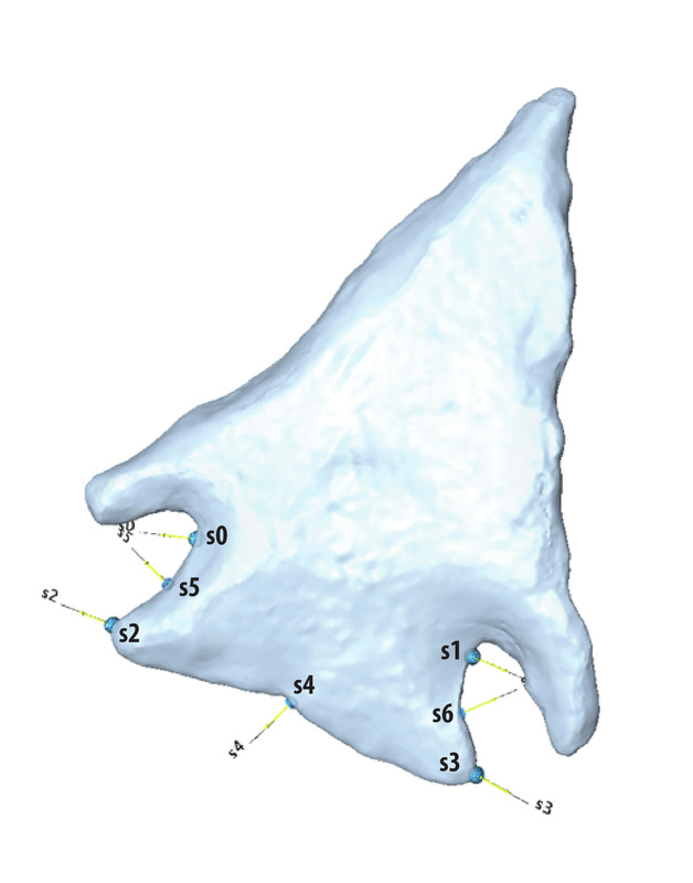
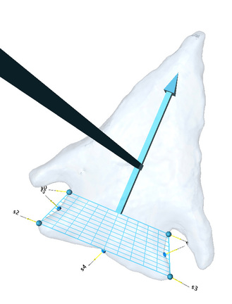
| I defined seven landmarks on each point (s0 through s6). To define these landmarks consistently, I first oriented the point to minimize the horizontal distance between s0 and s1. Generally, that resulted in s0 and s1 falling on roughly the same plane. I then defined s2 and s3 to mark the maximum deviation of the lateral haft edges proximal to maximum constriction of the haft (marked by s0 and s1). |
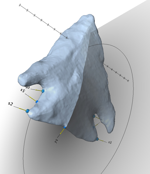
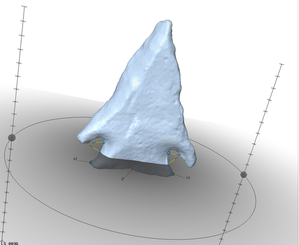
| I turned on the sagittal plane to locate landmark s4. The sagittal plane splits the axial plane down the middle. Landmark s4 is defined as the location where the sagittal plane intersects with the basal edge of the point when the sagittal plane bisects the axial plane. If the point is symmetrical, s4 will fall in the center of the basal edge. Note: the sagittal plane is movable. When you initially turn it "on," it's automatically centered in reference to the axial plane. If it gets moved you can recenter it simply by turning it off and then on again. |
I followed the same steps I described in the previous post to export and edit the data so that I could import it into MorphoJ. I used MorphoJ to perform a principal components analysis (PCA), the purpose of which is take all the variability in the 3D data and boil it down to its most important components. PCA lets you flatten the variability in a dataset into scores that you can plot in two dimensions.
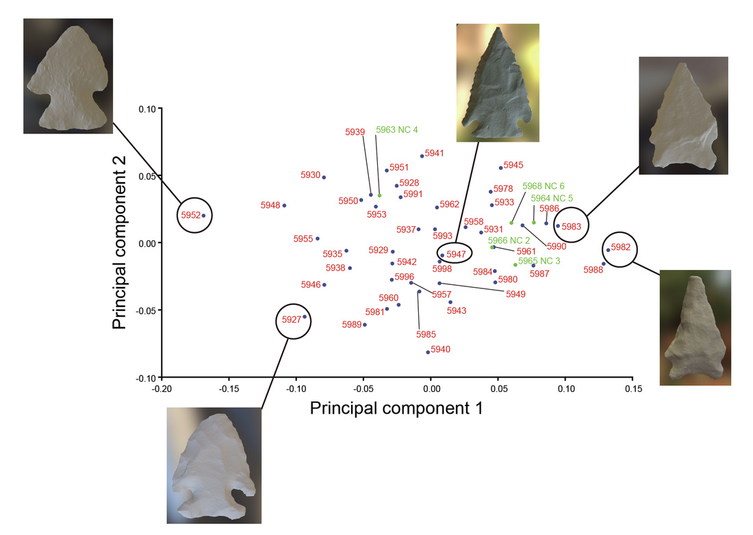
Here are the basic results of the PCA performed on the points currently in the sample:
With the exception of the Nipper Creek cache points (shown in green), all the points in the sample are from Allendale County, South Carolina, and are made from Allendale chert. This all but eliminates the possibility that the variability is due to space or raw material.
My next step is to explore the possible "time" component of the PCA by gathering some data from the point forms that bracket Kirk: Taylor (on the earlier side) and lobed/bifurcate points (on the later side). If I'm correct that the first principal component shown above is telling us something about time, the Taylor points should plot to the left and the bifurcate/lobed points should plot to the right. It's notable that four of the five points from the Nipper Creek cache plot close together. Those points were almost certainly produced during a short period of time (but so was 5963 NC 4, so . . . something to think about).


 RSS Feed
